16. OG-Core Output

16.1. Loading OG-Core output

When run, the OG-Core model saves model output in the baseline_dir and output_base files paths, which are set in the Specifications class object. For example (and this example assumes a certain directory structure that may not be the same on your computer):

     p = Specifications(
        baseline=True,
        num_workers=num_workers,
        baseline_dir="C:\User\OG-Core\Simulation24\Baseline",
        output_base="C:\User\OG-Core\Simulation24\Baseline",
    )

The baseline_dir argument refers to the path where the baseline output will be saved. The output_base refers to the path where the output for the given simulation (baseline or reform) will be saved. So in the example above, we are running the baseline simulation (hence baseline=True) and so we have baseline_dir and output_dir set to the same path. If this were a run of a policy reform, we would have a different path for output_base and baseline_dir would be the path to the baseline output. Even the reform run needs to know where the baseline_dir is because it will use the baseline solution to inform starting values for the reform simulation.

Within the baseline and reform directories, model solution outputs are saved for both the steady-state solution and the transition path. These will be in subdirectories with the structure:

baseline_dir
    |-- SS/SS_vars.pkl
    |-- TPI/TPI_vars.pkl
output_base
    |-- SS/SS_vars.pkl
    |-- TPI/TPI_vars.pkl

In each of the pickle files, one will find a dictionary object with the model output. The keys of the dictionary are the names of the variables and the values are the values of the variables. For example, the SS_vars.pkl file contains the steady-state solution values for the model variables. This dictionary is created in ogcore.SS.SS_solver. In the steady-state output, objects may be scalars, arrays of length S, arrays of length M, or arrays that are SxJ or SxJxI in dimension.[1] For the time path solution, the output dictionary is created in ogcore.TPI.run_TPI. Variables contained in this dictionary may be arrays of length T or multidimensional arrays of dimensions TxS, TxM, TxI, TxSxJ, TxSxJxI.[2]

To load one of these output dictionaries, one can use the pickle package in Python directly or the utility function in OG-Core, ogcore.utils.safe_read_pickle:

import pickle
ss_output = pickle.load(
    open("C:\User\OG-Core\Simulation24\Baseline\SS\SS_vars.pkl", "rb")
)

16.2. Interpreting OG-Core output

It is important to note that model output is measured in model units, which do not directly relate to units of GDP, either real of nominal. Because of this, and because the OG-Core framework is designed to simulation counterfactual analysis (and only secondarily to match a macroeconomic forecast) we prefer to interpret model output in terms of percentage changes between the baseline and reform simulations. For example, if one baseline and reform solutions for the steady-state with interest rates of 4% and 5%, respectively, it is often more useful to report results like “the model predicts that implementing reform X will increase the long run interest rate by one percentage point” rather than “the model predicts that implementing reform X will increase the long run interest from 4% to 5%.” The latter statement can be misleading because there are many assumptions underlying the long run interest rate of 4% in the baseline scenario, and economic forecasts may not even have such a long term horizon. Instead, by reporting percentage changes, we net out many of the assumptions underlying the baseline scenario and can more easily compare results across different economic forecasts (i.e., with and without the reform we are considering).

If you absolutely need to translate model output into nominal or real values, there are at least a couple options. In any case, it’s important to note that OG-Core is a real model (i.e., there is no inflation in the model) and the model output is stationarized. That is, the underlying population growth and economic growth in the model (summarized by the g_n and g_y parameters, respectively) is necessarily netted out when computing the model solution and all output is given in these “de-trended” values.

The first, and perhaps simplest, way to convert model output to nominal or real values is to find economics forecasts of the variables of interest and use these to scale the model output. For example, if you are interested in the movement of GDP, you could find a forecast GDP over some horizon and use use the model output to create an alternative forecast under the counterfactual reform scenario. For example, suppose the 10-year baseline forecast (in real of nominal units of local currency) for GDP is:

GDP_baseline = [100, 102, 104, 106, 108, 110, 112, 114, 116, 118]

And let’s suppose that the percentage difference in GDP between the baseline and reform simulations is:

GDP_diff = [0.01, 0.02, 0.03, 0.04, 0.05, 0.06, -0.01, -0.02, -0.03, -0.04]

Then the reform forecast for GDP would be:

GDP_reform = GDP_baseline * (1 + GDP_diff)
            = [101.00, 104.04, 107.12, 110.24, 113.40, 116.60, 110.88, 111.72, 111.52, 113.28]

A limitation of the the above approach is that it requires a forecast of the variable of interest. But given such a forecast, it is relatively easy to scale the model output to real or nominal units and you will have the model baseline match the forecast by construction.

A second approach is to take the model very seriously and scale model outputs directly to real world units. This involves two or three steps: (i) Add the trend back to the model output, (ii) convert the model output to units of local currency (in real terms), (iii - optional) turn the real units into nominal units by applying a price deflator. Let’s use GDP and an example again. The model output of GDP will be in TPI_vars["Y"], which is a one-dimensional array of length T. To add back the trend growth, one will need to multiple the series by the cumulative growth rates. What we want to get is:

\[Y_{t} = \prod_{u=0}^{t} (1 + g_{n,t}) * \hat{Y}_t * \exp(g_y * t)\]

Where \(Y_{t}\) is the nonstationary value of GDP and \(\hat{Y}_t\) is the model stationarized value of GDP.To compute this for the full vector of GDP in Python one would do:

non_stationary_Y = TPI_vars["Y"] * np.cumprod(1 + p.g_n) * np.exp(p.g_y * np.arange(p.T))

The next step is to convert the model output to units of real local currency. This is done by multiplying the model output by the value of factor_ss from the baseline steady-state solution. The factor_ss variable is used to convert model units to local currency since certain forms of the individual income tax functions are not scale invariant and thus since they are estimated in units of local currency, we need to make a conversion when applying them in the model.[^tax_scale_note] So to convert the model output to units of local currency, one would do:

local_currency_Y = non_stationary_Y * SS_vars["factor_ss"]

Finally, if one wants to convert the model output to nominal units, one would need to apply a price deflator. The price deflator would related to some forecasted inflation rate from outside the model. Assuming a vector of length T of forecasted inflation rates, pi, one would compute nominal values as:

nominal_Y = local_currency_Y * np.cumprod(1 + pi)

The advantage of this approach is that you can apply it to all the model outputs. The disadvantages include the complexity of the calculations and the factor that the model’s baseline solution may not match forecasts from outside the model. This might be a problem, for example, if there needs to be a consistent macroeconomic forecast from baseline simulations across a number of different models.

16.3. Summarizing OG-Core output

OG-Core has a number of useful tabulations and plotting functions that can be used to summarize model output. These are contained in the ogcore.output_tables and ogcore.output_plots modules. Note that some of the functions in the models are specifically for steady-state output, while others are for time path output. A few functions can accommodate both. For specifics of working with each of the functions in these modules, we refer the reader to the OG-Core API documentation. But we provide an example of interacting with one tabular and one plotting function below.

16.3.1. Tabular output

For some preset ways to view OG-Core output in a tabular format, see the ogcore.output_tables module. This module provides several table formats with options for output to be presented in different ways (e.g., as levels or percentage changes). The cell below shows how to read output and them use the ogcore.output_tables.macro_table function to create a table of percentage changes in macroeconomic aggregates between the baseline and reform simulations.

NOTE: the cell below runs in Python 3.10, but there’s an error reading the parameters pickle files in Python 3.11 that I could not figure out.

import ogcore.output_tables as ot
from io import BytesIO
import pickle
# import cloudpickle
import requests
path_dict = {
    "TPI": [
        "https://github.com/PSLmodels/OG-Core/blob/master/tests/test_io_data/TPI_vars_baseline.pkl?raw=true",
        "https://github.com/PSLmodels/OG-Core/blob/master/tests/test_io_data/TPI_vars_reform.pkl?raw=true"
            ],
    "Params": [
        "https://github.com/PSLmodels/OG-Core/blob/master/tests/test_io_data/model_params_baseline_v311.pkl?raw=true",
        "https://github.com/PSLmodels/OG-Core/blob/master/tests/test_io_data/model_params_reform_v311.pkl?raw=true"

    ]
}
output_dict = {
    "TPI": [],
    "Params": []
}
for key in path_dict.keys():
    for path in path_dict[key]:
        r = requests.get(path)
        output_dict[key].append(pickle.load(BytesIO(r.content)))
# make table
table = ot.macro_table(output_dict["TPI"][0], output_dict["Params"][0], output_dict["TPI"][1], output_dict["Params"][1], output_type="pct_diff", num_years=10, start_year= output_dict["Params"][0].start_year)
glue('pct_change_table', table.to_markdown())

Variable	2023	2024	2025	2026	2027	2028	2029	2030	2031	2032	2023-2032	SS
GDP (\(Y_t\))	0.242293	0.25705	0.26452	0.271852	0.280428	0.291875	0.30325	0.33648	0.353121	0.372514	0.298945	0.15837
Consumption (\(C_t\))	-0.101546	-0.0937955	-0.0920275	-0.0913839	-0.090299	-0.0887929	-0.0859871	-0.0884302	-0.0850751	-0.0814483	-0.0899271	-0.325536
Capital Stock (\(K_t\))	-0.167744	-0.159507	-0.147283	-0.130099	-0.108928	-0.0831552	-0.0543115	-0.0141228	0.0241502	0.0680466	-0.083661	-0.499739
Labor (\(L_t\))	0.095769	0.10457	0.109477	0.113299	0.116415	0.119352	0.121771	0.134597	0.138062	0.141778	0.119321	0.181081
Real interest rate (\(r_t\))	-0.675776	-0.48852	-0.419442	-0.389956	-0.380167	-0.386472	-0.395494	-0.455886	-0.476269	-0.504356	-0.446212	0.000497603
Wage rate	0.143909	0.149049	0.150991	0.15375	0.158361	0.165692	0.173687	0.189133	0.200724	0.214481	0.17112	-0.0431336

16.3.2. Plotting output

OG-Core also offers functions for easily visualizing output. These functions are available in the ogcore.output_plots module. This module provides a number of different types of plots with can be used to visualize macroeconomic aggregates, household decisions, and customized to plot different variables in different units. The cell below shows how to read output and them use the ogcore.output_tables.plot_aggregates function to create a table of percentage changes in macroeconomic aggregates between the baseline and reform simulations.

NOTE: the cell below runs in Python 3.10, but there’s an error reading the parameters pickle files in Python 3.11 that I could not figure out.

import ogcore.output_plots as op
from io import BytesIO
import pickle
# import cloudpickle
import requests
path_dict = {
    "TPI": [
        "https://github.com/PSLmodels/OG-Core/blob/master/tests/test_io_data/TPI_vars_baseline_v311.pkl?raw=true",
        "https://github.com/PSLmodels/OG-Core/blob/master/tests/test_io_data/TPI_vars_reform_v311.pkl?raw=true"
            ],
    "Params": [
        "https://github.com/PSLmodels/OG-Core/blob/master/tests/test_io_data/model_params_baseline_v311.pkl?raw=true",
        "https://github.com/PSLmodels/OG-Core/blob/master/tests/test_io_data/model_params_reform_v311.pkl?raw=true"

    ]
}
output_dict = {
    "TPI": [],
    "Params": []
}
for key in path_dict.keys():
    for path in path_dict[key]:
        r = requests.get(path)
        output_dict[key].append(pickle.loads(BytesIO(r.content).getvalue()))
# make table
fig = op.plot_aggregates(output_dict["TPI"][0], output_dict["Params"][0], output_dict["TPI"][1], output_dict["Params"][1], plot_type="pct_diff", start_year= output_dict["Params"][0].start_year)
glue("pct_change_agg_fig", fig, display=False)

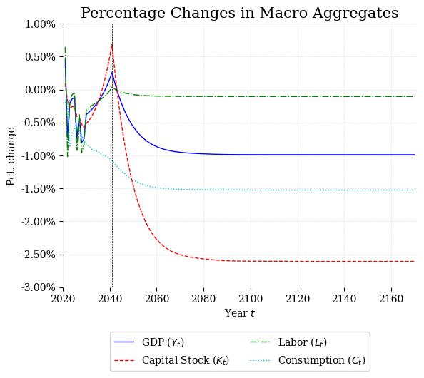
Fig. 16.1 Percentage Changes in Macroeconomic Aggregates

16.4. Exercises:

Exercise 16.1

Solve for the steady state of the model with the default value for the rate of time preferences (this is \(\beta =0.96\)). Then solve for the steady-state solution with \(\beta=0.90\) (remembering to save the output in a different location than your baseline simulation). Use the ogcore.output_plots.ss_profiles function to plot savings by age over agents lifetimes before and after the change in the rate of time preference. What do you notice happens to savings?

Exercise 16.2

Take TPI output from https://github.com/PSLmodels/OG-Core/blob/master/tests/test_io_data/TPI_vars_baseline.pkl and convert the GDP series to constant units of local currency using the factor_ss and the growth rates, g_n and g_y. You can find the factor_ss in the steady state output at https://github.com/PSLmodels/OG-Core/blob/master/tests/test_io_data/SS_vars_baseline.pkl and the growth rates in the parameters file at https://github.com/PSLmodels/OG-Core/blob/master/tests/test_io_data/model_params_baseline.pkl Hint: you can look at the OG-Core chapter on stationarizing the model to help see how to get back to non-stationary measures.

For the next three exercises, you are going to need to use time path output from a baseline and reform run and the corresponding parameters. You can download these from the following links:

• Baseline TPI output: https://github.com/PSLmodels/OG-Core/blob/master/tests/test_io_data/TPI_vars_baseline.pkl

• Baseline parameters: https://github.com/PSLmodels/OG-Core/blob/master/tests/test_io_data/model_params_baseline.pkl

• Reform TPI output: https://github.com/PSLmodels/OG-Core/blob/master/tests/test_io_data/TPI_vars_reform.pkl

• Reform parameters: https://github.com/PSLmodels/OG-Core/blob/master/tests/test_io_data/model_params_reform.pkl

Exercise 16.3

Use the ogcore.output_tables.macro_table function to create a table that shows differences by year between macro variables in the baseline and reform model solutions.

Exercise 16.4

Use the ogcore.output_plots.plot_aggregates function to create a figure showing the percentage changes in GDP and consumption over the transition path between the baseline and reform simulations.

Exercise 16.5

Now use the ogcore.output_plots.plot_aggregates function to plot the baseline GDP forecast and the what that forecast (in levels) would look like under the reform scenario. This will involve setting the plot_type="forecast" and passing in an array that is the baseline GDP forecast (you can make this up or find a real forecast online - just note that the length of this array needs to be equal to the argument for num_years_to_plot, which defaults to 50 but can be adjusted).

16.5. Footnotes

The footnotes from this chapter.

---

[1]

Recall that S refers to the maximum number of model periods an individual may be economically active and J refers to the number of ability types. The number of production industries is given by M and the number of consumption goods by I.

[2]

The number of periods in the transition path is given by T. [^tax_scale_note] This is done in functions in the ogcore.tax module. The value of factor_ss is endogenous and is solved for in the steady-state equilibrium by finding the value of the factor that makes the mean household income in the steady-state solution equal the mean household income from data used to estimate the tax functions.