17.1. Demographics#
A key feature of OG models is the ability to model the impacts of economic shocks or policy changes across generations. Because they capture generations of finitely-lived agents, OG models can be made to reflect realistic demographics. Demographic trends are of massive importance to economic trends. Furthermore, there is a tremendous amount of variation in demographic trends across countries. Consider Figure 17.1, which shows the population distributions, and their evolution over time, for three countries: South Africa, India, and the United States. In each figure, we plot the 2023 population distribution (according to data from the UN World Population Prospects) and then the evolution of the population as we age it forward two, 40, and 80 years and then to it’s steady state distribution using the demographics.py module from OG-Core. Comparing the 2023 distributions first, we see that South African distribution has humps, which reflect the initial wave of the HIV epidemic and then it’s echo on the next generation. We see also that India has more young adults than the two other countries, but displays a relatively flat gradient as the number of individuals decline quickly with age, reflecting relatively high mortality rates in that country. The United States has a more right skewed distribution than South Africa and India, with more individuals of advanced age, reflecting relatively low mortality rates for adults. As each population is simulated forward in time, we see the age distribution move to the right, with older individuals representing a larger share of the population in each country. After about 40 years, these populations are very close to their steady-state. Since older individuals make significantly different labor supply and savings decisions than young individuals, these evolutions of the population will have profound effects on wages, interest rates, and economic growth.
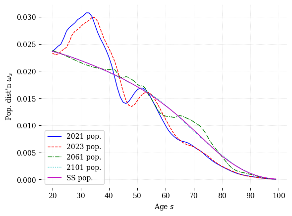
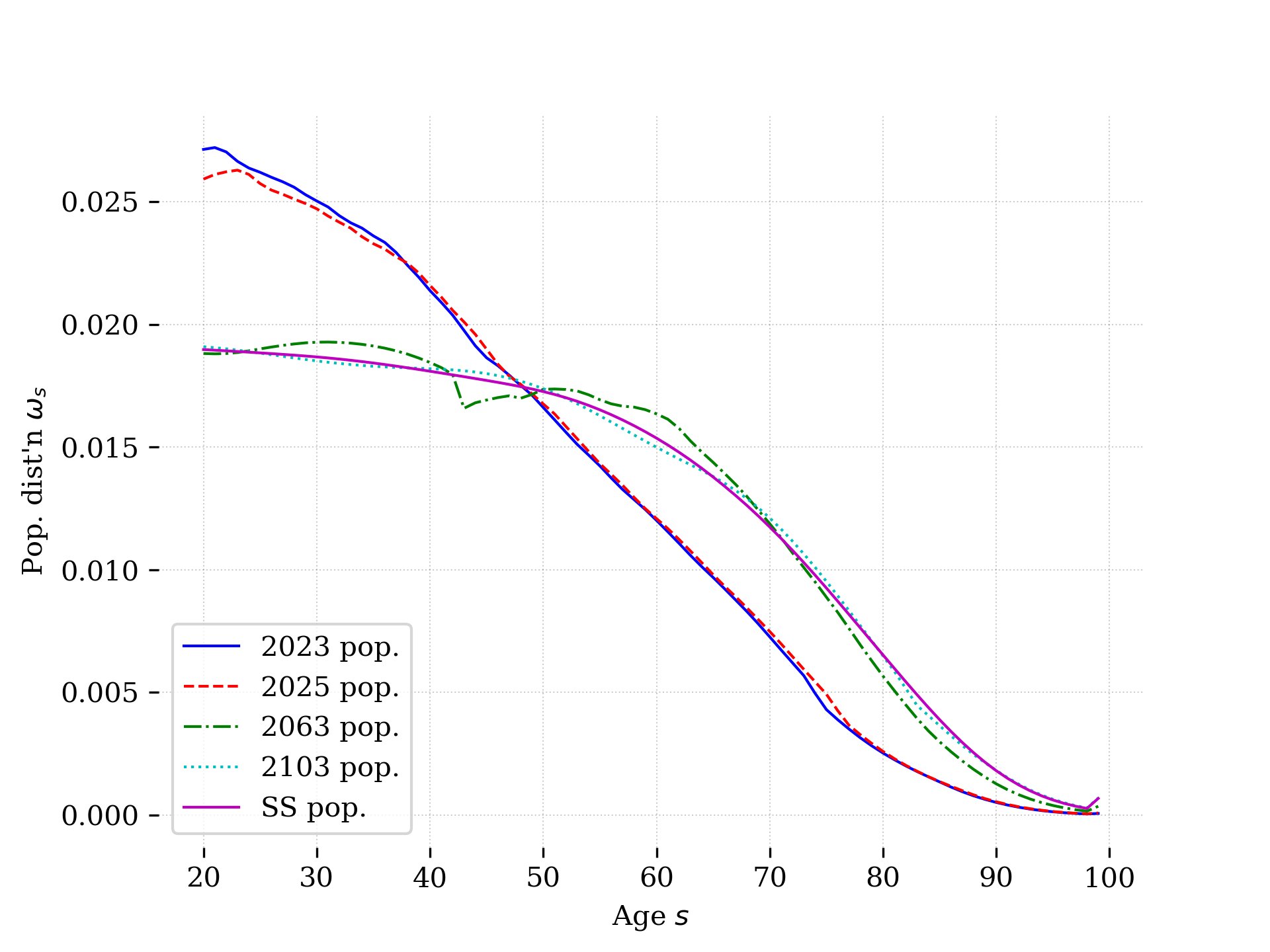
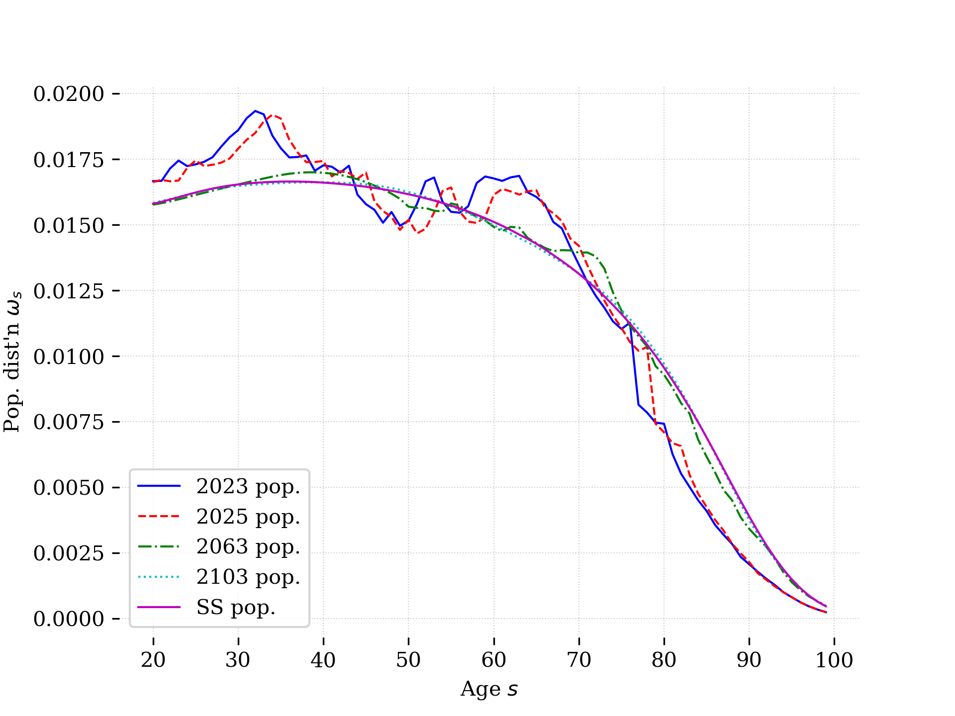
Fig. 17.1 Population distributions in South Africa, India, and the United States#
Figure 17.2 plots population growth rates over time for the three countries illustrated above. The growth rates are determined by the same mortality, fertility, and immigration trends that drive the evolution of the population in Figure 17.1. In terms of population growth, we see that in all countries the population growth rate is declining in each of the three counties over the next 60 years. This is consistent with what we saw in the evolution of the population distribution in the three countries above: each economy is aging and with relatively more older individuals, total fertility will be declining. Looking at the level of population growth in the long run in Figure 17.2, we see that India and the United States will have negative population growth, which will put downward pressure on their long run economic growth rates. In contract, South Africa will have positive population growth, owing to it’s relatively high fertility rates, which will contribute positively to that economy in the long run.
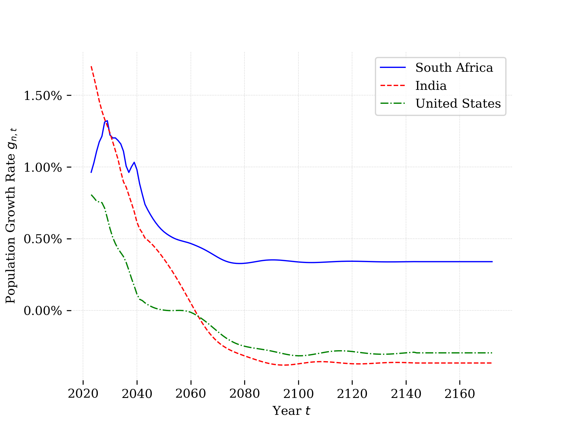
Fig. 17.2 Projected time path of population growth rates in South Africa, India, and the United States#
The population distribution and growth rates in the plots above were created using the demographics.py module from OG-Core. Each of these country calibrations utilizes population data from the UN World Population Prospects database, which provides consistent data on the population distribution and age-specific mortality, fertility, and immigration rates by country for many countries. Note that although immigration rates are provided in the UN data, they are not given by age and the demographics.py module imputes them as the residual between the population counts by age and what would be expected given the measured fertility and mortality rates. This is done for two reasons. First, it ensures that the evolution of the distribution of population by age is consistent with the three forces affecting it: fertility, mortality, and immigration. Second, it is difficult to accurately measure immigration since not all immigrants are documented (with substantial variation in this across country). Using the residual method to identify immigration may therefore be more accurate than official statistics.
demographics.py has several functions within the module. You can find a summary of those functions in the OG-CoreAPI documentation. Below we offer several exercise that have you interact with this module help you learn better understand its inputs and outputs.
17.1.1. Exercises#
Exercise 17.1
First, let’s gather population data from the UN Population Prospects for a country of interest to you. You can do this by calling the ogcore.demographics.get_un_data function. This function takes one positional argument, the UN variable code, and three keyword arguments, the country code, the start year, and the end year. The UN variable code is a string that identifies the data you want to pull from the UN database. The country code is a string that identifies the country you want to pull data for. The start year and end year are integers that identify the range of years you want to pull data for. The function returns a pandas DataFrame with the data you requested. Use this function to pull data for a country of interest to you. You can find the UN variable codes and country codes in the UN Population Prospects documentation. Because the UN has an API token for data access, please select a variable code from “68” (fertility rates), “80” (mortality rates), or “47” (population by age) for this exercise. Also choose a country code from the following list: “840” (United States), “710” (South Africa), “458” (Malaysia), “356” India, “826” (United Kingdom), “360” (Indonesia), “608” (Philippines). Note that the maximum year value is 2100. Also note that retrieving data will require an internet connection you will be prompted for an API token, but if you don’t have one, just hit enter and the function will still work.
Exercise 17.2
Using your modified demographics.py, plot the fertility rates in this country. Note that you can do this directly from the demographics.get_fert() function.
Exercise 17.3
Let’s do the same for mortality rates. In this case, you will want interact with the demographics.get_mort function.
Exercise 17.4
The demographics.py module uses current fertility and mortality rates (and the implied immigration rates) to project the population forward. This ensures a population distribution in each year of the model that is consistent with the fertility, mortality, and immigration rates. Use the demographics.get_pop_objs function to return a dictionary with the population object that are inputs to calibrating OG-Core (Use E=20, S=80, T=320, curr_year=2023). From this dictionary, extract the population distribution object (the key for this is omega and it is an array with shape TxS, where T are the number of time periods and S is the number of age groups in the model). Create a line plot of the population distribution in the first year, the 20th year, the 100th year, and the last year in the omega object. Describe what you see happening to the distribution of people across age as you more forward in time?
Exercise 17.5
Also in the dictionary returned from demographics.get_pop_objs, is the population growth rate. This is a NumPy array object with key g_n. Plot g_n. How does the population growth rate change over time? Given what you’ve seen in the plots you’ve created, what can you say about the driver(s) of population growth (i.e., how are fertility and mortality rates contributing? What about immigration (something we haven’t yet plotted, but about which you might be able to infer something given fertility and mortality rates and the change in the age distribution over time…))
Exercise 17.6
Now that you’ve visualized the different demographic trends in the country you’ve chosen, let’s see how these affect the equilibrium in the OG model. This will combine what you learned in Simulating OG-Core with what you’ve learned here about population demographics objects for the model. You’ll proceed with the following steps:
Instantiate a
Specificationsclass object fromOG-Corewith:p = Specifications( baseline=True, baseline_dir=base_dir, output_base=base_dir, )
where you set the directory you’d like this output saved with a string base_dir.
Use the
ogcore.execute.runner()function to solve for the steady state of the model.Now, create a new Specifcations object with:
  p2 = Specifications(
        baseline=False,
        baseline_dir=base_dir,
        output_base=reform_dir,
    )
where you set the directory you’d like the output from this second model run saved with a string reform_dir.
Use the demographics module you edited above to return the a dictoinary of population objects from
demographics.get_pop_objs. Use these to update thep2object:
p2.update_specifications(pop_objs_dict)
Use
ogcore.execute.runner()to solve the model again, this time with the parameters inp2.Finaly, comparet the differences in the steady-state macroeconomics variablkes using
ogcore.output_tables.macro_table_SS. What do you see? How did demographics affect aggregate output? Wages? Interest rates? Do you have intuition about why this happened?