17.4. Earnings Processes#
An important component of the OG-Core model are the household earnings processes. These help to match real difference across age and households in earnings ability and are a key set of parameters to model income inequality. Household earnings are endogenous and depend on the households’ decisions to work and save given the state of the economy and household preferences and ability. What is exogenous to the model are how productive households are with each unit of labor they supply, i.e., their earnings ability. OG-Core assumes that there are J groups of households with different earnings abilities. Within each group, the earnings ability process is deterministic and known to the household, although labor productivity of these workers vary over their working life. Fore example, consider Figure 17.3, which shows the log of effective labor units for each of seven lifetime income groups, estimated in the United States. Each group is defined by their “potential” earnings over their lifetime (i.e., if they worked full time, what would they earn over a 40 year career) and grouped by their percentile rank in the distribution of lifetime incomes. We can see that the top 1% of lifetime earnings have higher productivity in each year of working life, but because productivity varies with age, this gap is not constant. Rather, it’s largest during the peak earnings year of middle age and then is quite small at older ages.
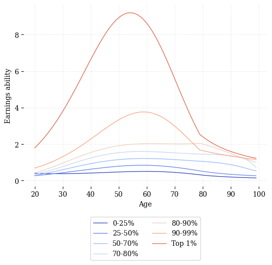
Fig. 17.3 Log Effective Labor Units by Lifetime Income Group, Estimated in the United States#
In OG-Core, these earnings processes are described by SxJ matrix, with each cell representing the effective labor units for a given age and lifetime income group. Note that this matrix is normalized such that the average value of earnings ability is one. It is assumed that these processes remain constant over time, so despite growth in the level of productivity through the exogenous technological growth,
To estimate the earnings processes in Figure 17.3, we used administrative data from tax returns the covered a panel of US taxpayers over four decades. A detailed description of this process is given in the OG-USA documentation. Suffice it to say, this estimation process is quite involved and requires a large panel dataset in individual or household earnings, ideally without censoring the top end. In many contexts, these data may not be available. We therefore will describe here an approximation technique that is less data intensive, and leave the more involved estimation process for the interested reader to explore in the OG-USA documentation.
To approximate the earnings processes in a country of interest, we recommend starting with the OG-USA calibration and then applying a transformation to these earnings processes to match the distribution of income in the target country.[1].
17.4.1. Exercises#
Exercise 17.11
Use income.py from OG-USA to retrieve the earnings process matrix. Read through the docstrings of each function to see which to use. With the e matrix that is returned, create a line plot of the earnings at each age for the J different types.
Exercise 17.12
Now we’re going to adjust the above earnings process to match the Gini coefficient in a country that isn’t the U.S. (note that the Gini coefficient for income in the U.S. was 41.5 in 2019). The transformation we’ll make is:
where \(C\) represents the country of interest. We will find \(a\) by matching the Gini coefficient in the country of interest. To do this, we’ll use the scipy.optimize module. First, create a function that takes \(a\) as an argument and returns the Gini coefficient in the country of interest (hint: the ogusa.utils.Inequality class object will be helpful here). Then, use the scipy.optimize.minimize_scalar function to find the value of \(a\) that minimizes the difference between the Gini coefficient in the country of interest and the Gini coefficient in the U.S. Finally, use the value of \(a\) you found to transform the e matrix from the U.S. to the country of interest. Plot the earnings processes in the U.S. and the country of interest. How do they differ?
17.4.2. Footnotes#
The footnotes from this chapter.